Every time I load a new set of film scans into my editor, I feel like I have to start from scratch. Or anyway it feels like I learn something new about my process with each roll. So far it has been a lot of fumbling around, a lot of fits and starts.

What I really want is a clear, objective way to understand the way the film I shoot behaves. I want to know how to reliably, repeatably move from selecting a film and speed, exposing a frame, developing the film, scanning the film, and producing a finished digital image—without bumbling around, or guessing, or making things up from scratch every time I do a new scan.

Here’s the thing. I could buy a densitometer and turn my home office into a precision film lab. But that’s expensive and time consuming. I don’t want that. Moreover, the usual way for performing these evaluations is geared towards making darkroom prints. I make digital scans. I want a workflow that supports my goal of producing digital works.

So, after a great deal of planning and thinking, I’ve got a new system. Although I might be getting ahead of myself, I think it’s working pretty well for getting better images from my film, from exposure to final digital editing. The best part is if you want to try it for yourself, you can follow along at home—you only need a computer monitor, a way to scan film, and a spot meter you trust.

Background

Inspired by recent weirdness I experienced with AgfaPhoto APX400, I decided to get systematic about things. Previously, I had been using a Datacolor Spyder Checkr 24 calibration target to get a feel for how a film is behaving. But, checking out the gray targets with a spot meter was a little disappointing.

There are six gray targets on the Spyder Checkr 24:

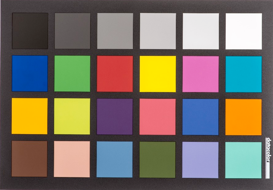
If I meter the black one to Zone 0, then moving from left to right I measure:
0, I, II, II.5, III, III.5
which is a little disappointing. I'd like a target with a fuller dynamic range. A huge part of the problem is quite simply that I have no way of shining a brighter light on the target in a consistent way.

So while I still think that’s useful for understanding the spectral response of a film, I decided I could do better for measuring the tonal response.

Something Better?

Aside: There is a solid chance that I am getting ahead of myself. I’ve only put one film through this process, after all. But I think I might be on to something, I think it’s already been helpful for me, and I’d like to know if it’s helpful for you.

After pondering the light source issue I described above, I realized that I do have a consistent and bright light source I could use…my computer monitor. I can't use it to illuminate, but I can use it to display a digital target. Best of all, it has nearly ten stops of dynamic range (it’s listed as having a 1:1000 contrast ratio, which is pretty close to reality—yours might well be at least this good, maybe even better!)

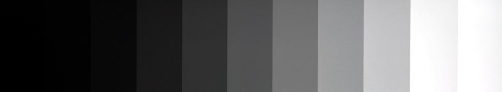
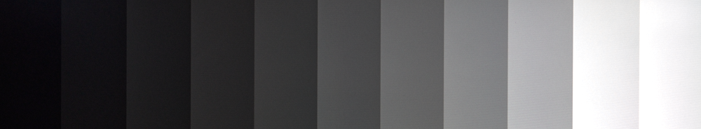
So, in broad strokes, my new method is now this: I take a photo (perhaps bracketed for exposure) of a carefully calibrated digital target on my computer monitor, like this:

I can take photos of this target directly on my monitor to estimate the speed of my film, to evaluate the development process, and to automatically correct the exposure and contrast for each frame (to a reasonable starting point, anyway).

Set Up

Notice the words “carefully calibrated”. There is some work to do up front. Please don’t use the image above as is. The reason is that monitors have a built-in contrast curve. Flat contrast is boring, and also a little weird looking, so nearly all monitors up the contrast a bit, compressing the darkest and lightest tones in the process. We need a way around that for this to work. And I don’t believe in relying on mathematical models and theory to get this right—we’re going to calibrate everything by hand, with a light meter.

Set up your monitor

This part is simple, because we’re not going to rely on the monitor’s own calibration (or lack thereof), instead compensating for it in other (and cheaper) ways. Just make sure your brightness is set to full, and the contrast to half. This should allow it to produce the widest dynamic range possible.

Calibrate the test target

Now, here is a file I created. You will not be able to use it as is—it has been calibrated for my own monitor. But the calibration process isn’t difficult, and you don’t need special software. This is an HTML file—it’s a text file you can edit in a basic text editor like Notepad or TextEdit, but it is also contains an image file you can display in your favorite web browser..

Download the HTML file below, and open it with your favorite web browser—it’ll know how to display the image.

At the same time, open it in a text editor like Notepad or TextEdit. Don’t feel overwhelmed if you don’t understand what all is going on: Although it needs editing it won’t need much.

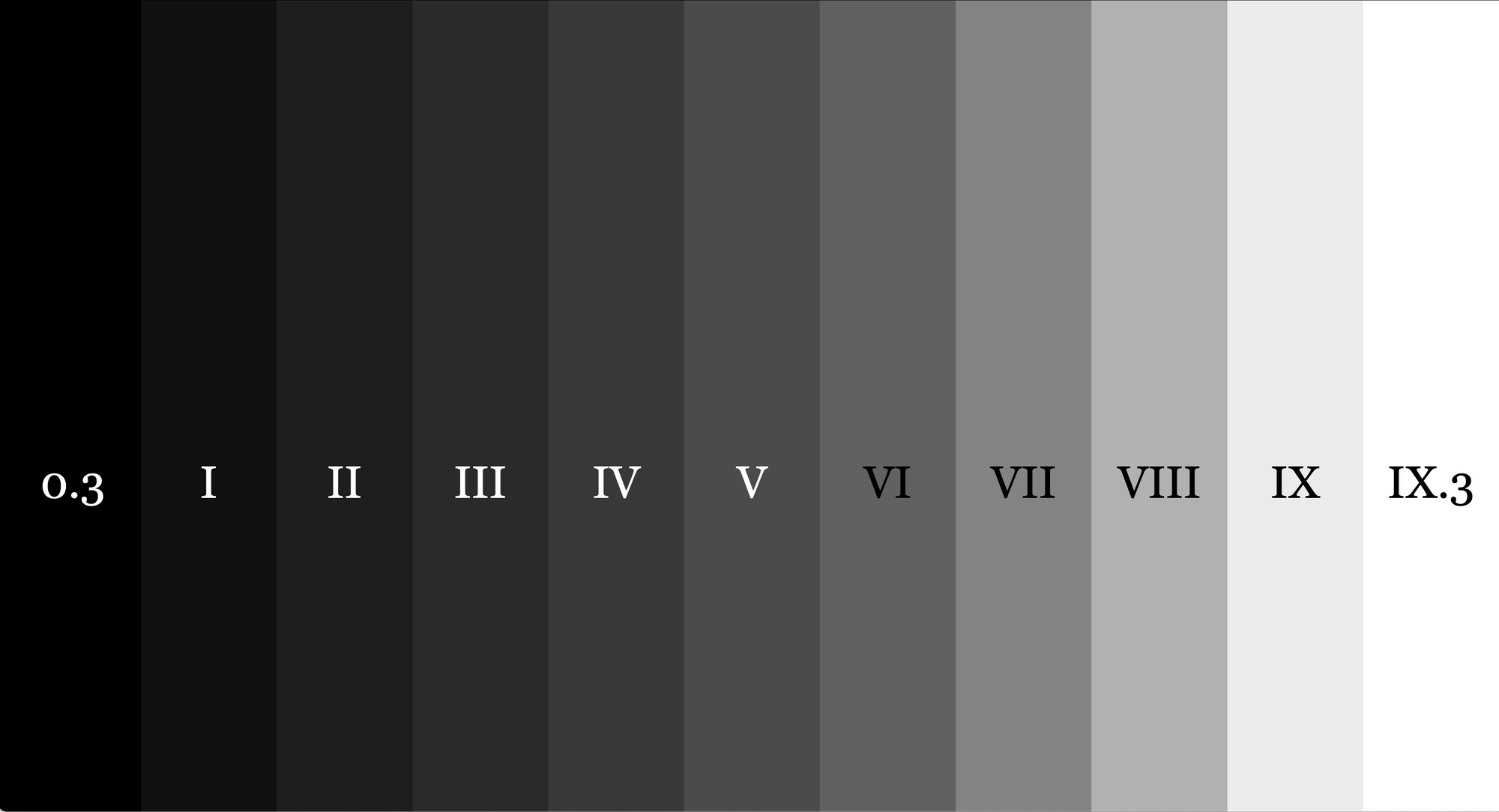
Do you see the eleven repeating elements labeled “tone samples”, and labeled with the 9 different Zones in Roman numerals? Notice how each of those elements has a color associated with it in the notation rgb(x,y,z) (or in the case of pure white and pure black, a color name). We’re going to use our spot meter to get the correct values for zones I–IX.

Turn out the lights, close the window shades, and pull out your spot meter. Meter each of the zones in the image. On my setup, pure black, Zone 0, meters at EV100 1.3. This is not a convenient value, as the recommended camera settings aren't possible on my equipment—this is why I decided not to represent Zone 0 on my own chart, relegating it to “0.3” instead. With my cameras, I can reliably set values that correspond to whole-valued EVs, and since I can’t make pure black any darker, I just started from Zone I.

When you meter Zone I, you might get all kinds of different values. What you want to meter is something at a full EV100 value, and just brighter than what you metered for Zone 0. In my case, I meter that zone at EV100 2. But you might meter it at something different. This is where we have to edit.

In your text editor, adjust the numbers for Zone I up or down. The three values represent red, blue, and green, so to get gray they all must be the same. The default is a gray value of 16 (out of 255). If you need to make it somewhat lighter, change this:

.I {
  fill: rgb(16,16,16);
}

to this:

.I {
  fill: rgb(20,20,20);
}

The change from 16 to 20 is just a number I made up. Larger values are brighter, lower values are darker. You’ll have to find the right number that gives you a good whole-number meter reading. Save the file, and reload your web browser. You should see the updated value. Take a new meter reading, and repeat until Zone I is dialed in.

Once you have Zone I dialed in, continue to Zone II. The meter reading should be one full stop brighter. Again, you’ll need to adjust the tone value in your text editor, save, and reload your web browser. Keep this up until you get to Zone X, or you reach a Zone whose value exceeds 255. 255 represents pure white, and you cannot go brighter than that!

In my case, I was able to get to Zone IX without capping out at 255. But I couldn’t get Zone X to be a full stop brighter than IX—it was only a third stop brighter, so I labeled it “IX.3” for clarity.

Bonus: You can also update the labels to reflect what you were able to achieve with your monitor. Just look for these elements:

<text x="1.5" y="11" text-anchor="middle" class="label white">0.3</text>

And change the bit just before </text> to alter the label.

Calibrate scanning camera

OK, so now you have your monitor displaying a test target with distinct zones, all (more or less) one stop apart in brightness! We’re nearly done. If you use a flatbed scanner, you are totally done and can skip this step.

If like me you use a digital camera to make film scans, we have a little bit more work to do. Specifically, we need to figure out how to get a true linear response from our raw files. As it happens, even when using a linear profile for processing raw files, the results are not linear enough. So we need to compensate a bit. This part is more art than science, to be totally honest.

Additionally, I don’t know how to do this in any software other than Capture One. If you have an idea how to do this in Lightroom, I would love to hear from you!

First, take a screenshot of your new test target, and load that screenshot into your editor. We’re going to need this to see how far off our camera’s contrast curve is from ideal.

So, display your new test target. Meter the target with your spot meter for Zone V—don’t trust your digital camera’s built-in meter for this. Then take a picture! Include the whole test target.

Now, the results may not look like the original image, and that’s expected. We just have a little adjustment to do.

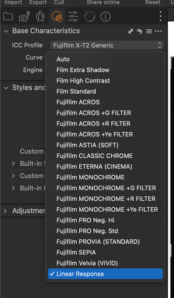
First, we need to make sure that our image editor is using a flat or linear contrast curve to process the raw file. In Capture One, this is in the ICC Profile under the Base Characteristics tool. Make sure it is set to “Linear Response”.

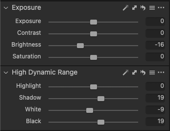
In Capture One, the Exposure and the High Dynamic Range settings are applied before Levels and Curves. I don’t usually use the Exposure and High Dynamic Range settings when editing a film scan. Which makes them perfect for this next adjustment. We want to make the grays in the photo we just took match the original image as closely as possible.

My goal was to make sure that Zones II, V, and VIII were as closely matched as possible to the test target. I moved Zone V by adjusting the brightness (which moves tones in the middle without messing with tones at the extremes), and then adjusted the HDR sliders to align the shadows around Zone II and the highlights around Zone VIII. The results are not perfect, but it is really close. Here is what I ended up with, your results will vary:

Notice that Zone V isn’t in the middle of the histogram! And that there is a lot of unevenness in the distribution of the tones across the histogram. Don’t worry about this. Everything was calibrated with the spot meter earlier, and this step is just to make sure that the tones in our film are reproduced accurately on our monitor for editing later. Trust the process.

I saved these settings to a preset that I can load up and apply on demand, without having to remember all those values. (Or anyway, I tried to. Capture One is being weird about loading my presets at the moment, and I’m stuck debugging this part of the process. But in theory, it should work like that.)

Output

So, at this stage, we have two things:

1. A calibrated test target that works on our monitor.
2. A calibrated preset for our digital camera so the scans come out as flat as possible.

Now it’s time to put these tools to use!

The System in Use

The upfront work to calibrate everything is the hard part. Now things get a bit simpler. The process here is straightforward: Photograph the test target, then scan as usual.

Making a test image

Turn up the music. Turn off the lights. Display the test target full screen. Meter the target at Zone V using your spot meter. Load up the film stock you want to analyze, and take a photo. Better yet, bracket a set of photos at different exposures. If you are evaluating a film’s true speed, definitely bracket.

Then, finish the roll as you normally would, and develop!

Establish black and white points

Actually first, we need to establish the full dynamic range of the film. We can find the darkest possible tone in the clear film base, and the brightest possible tone in the fully-fogged film leader (If you’re shooting medium format, you might need to—shudder—sacrifice a frame to the gods of light, since you don’t have a leader).

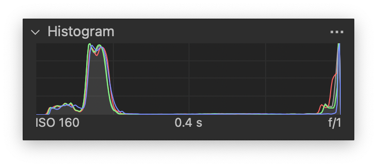
Then scan the fully fogged leader together with an unexposed portion of the film. Don’t forget to use a linear response for the raw processing options, just as above! Adjust your scanning exposure to get both pure white and pure black, and pushed as far apart in the histogram as possible, without clipping.

In my case, this is almost universally ISO 160, f/5.6, and 1/2.5s. Your results will vary.

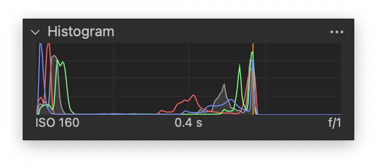
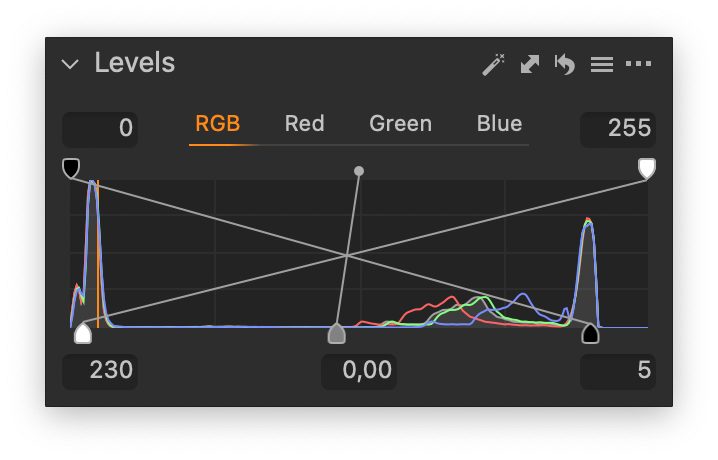
Because we’re dealing with negatives almost certainly, we need to invert the image, so the highlights render as white and the shadows as black. In Capture One, we can do this with the Levels tool, by sliding the white and black points to the opposite end of the spectrum. If you’re scanning positives, don’t bother with the inversion.

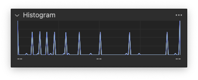
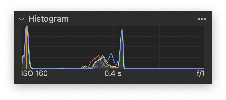
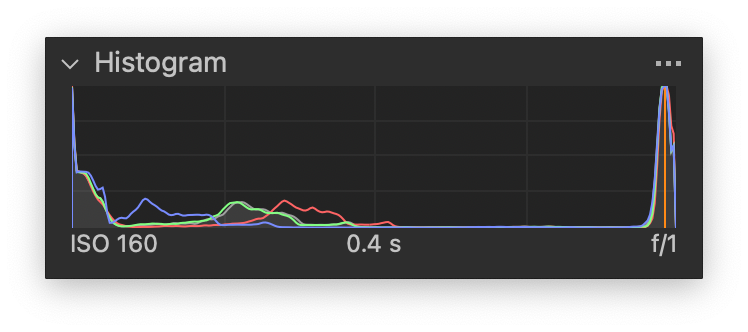
Then, we need to adjust the white and black points to match the film. Slide the white point to the right just under the spike in the histogram; do the same with the black. Your results will look something like this:

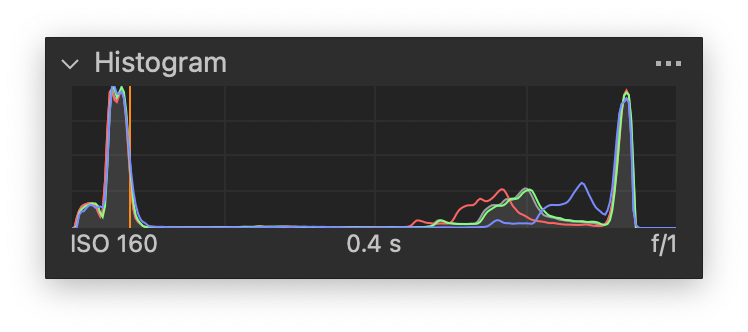
And here is the final histogram. (Ignore the small peaks near the middle, this is an artifact of the way I scanned the film leader. We only care about the extreme highlights and shadows.)

Scan the image of the test target

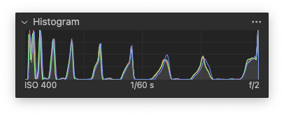
Now, the part we’ve all been waiting for. Using the settings established above—linear response, camera response preset, and target levels—scan the photos of your test targets. Here, I am evaluating the speed of AgfaPhoto APX400. I shot the first frame at ISO 200, the second at 400, and the third at 800.

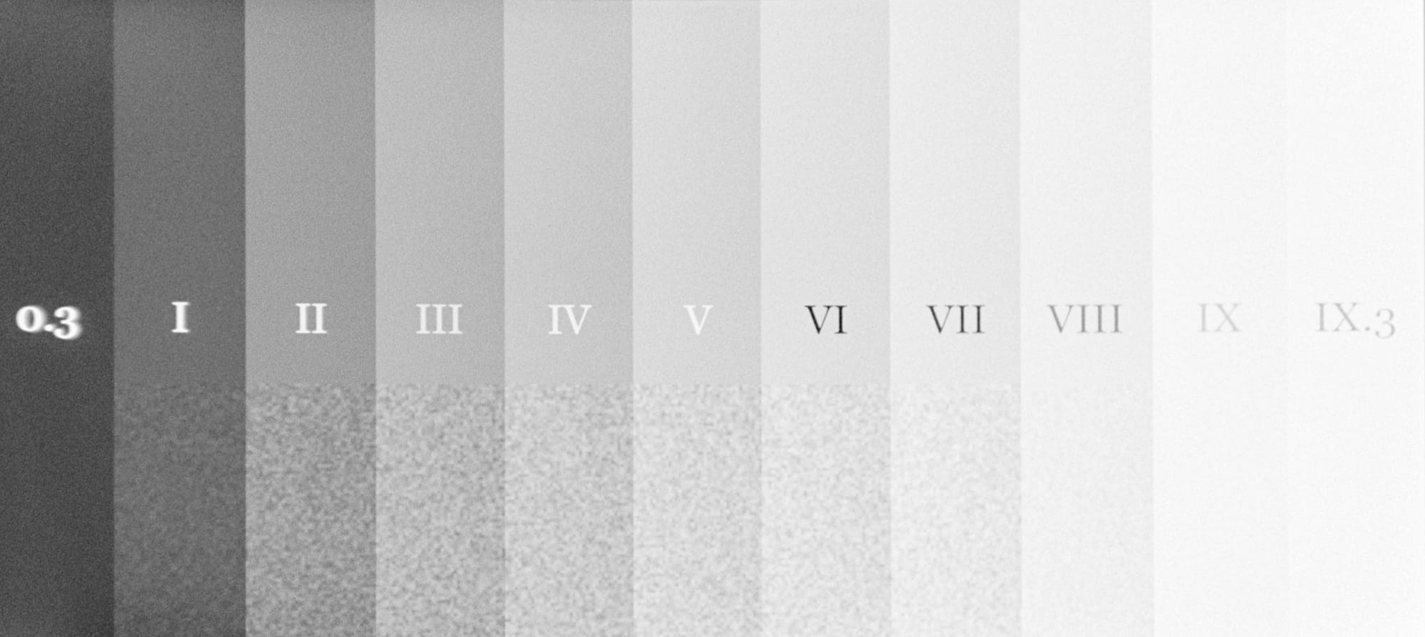
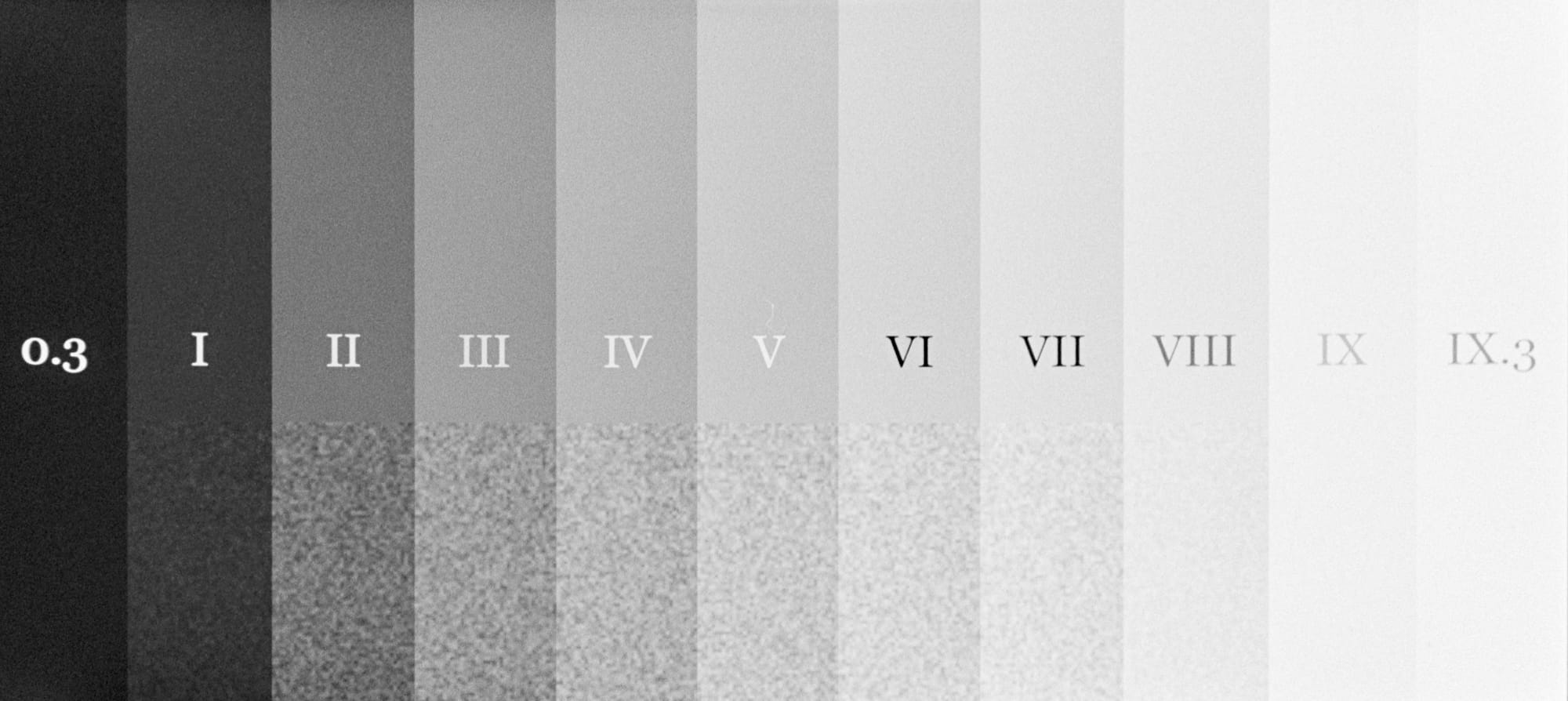
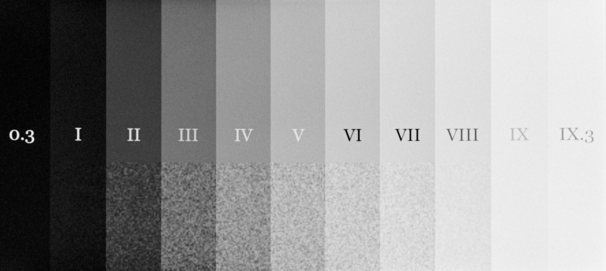
(Ignore the fact that these images have some digital noise added—I decided this wasn’t as helpful as I thought it might be, and removed it from the final version I am sharing in this post).

I interpret these results in more detail in a separate article, but the main takeaways are clear to see.

At ISO 200, the shadows are simply too bright. This is an over-exposed frame.

At ISO 400 the shadows are improving, but they are still too bright. Zone 0.3 should be essentially black, and Zone I should not show much if any texture, and should be just distinguishable from black.

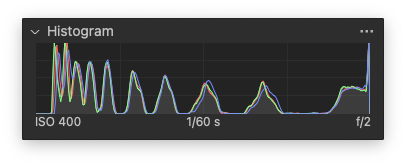
At ISO 800, the shadows are exactly where they should be, which is why (given my development process) I believe this film to have a true speed of 800. The contrast is a little flat, which makes me think there is room to push this film to at least 1600, possibly 3200 with good results.

In all the images, the highlights reach about the same level of brightness—and that’s not very bright. I suspect under development, but more experimentation (and more experience with this system) will be necessary to say for sure.

We can also use a tool like Apple’s Digital Color Meter app to evaluate the digital tones at each zone, and construct a digital characteristic curve:

You can see more graphically the really low contrast from the midtones to the highlights that led me to think this is under developed!

Conclusion

I’ve presented here a new system for evaluating film, analog process, and digital process to assist in the creation of digital images of the highest quality from black and white film stock. It’s still new for me! I have a lot of exploration to do to see if it will help me achieve my goals.

I hope that you will try it out, that my instructions are clear enough to reproduce my results. Please leave questions and comments in the comments below!

I for one certainly intend to apply this tool to every new combination of film, developer, and speed—and to share those results here. Look forward to it!

Support this blog

If you enjoy reading this blog, I encourage you to consider purchasing a book or print to show your support. And if you're into analog photography, check out my new mobile app Crown + Flint.

Books & Prints

Photographs are best appreciated in print. Get your own printed editions of my photographs and support my work by buying a book or print for yourself or as a gift. Loading…

Don Goodman-WilsonDon Goodman-Wilson

Crown + Flint

The digital companion for your analog lifestyle. Improve your analog technique, capture shot metadata, manage your film collection.

Crown + Flint